
- Jul 9, 2021
- 13 min read
Written By
- Francesco Lässig
In the following article we will discuss the topic of Anomaly Detection and Transaction Data, and why it makes sense to employ an unsupervised machine learning model to detect fraudulent transactions. We will discuss the Dataset used, and go through all the steps from Feature Engineering to choosing and building the right Model for the task at hand. Next, we will evaluate the Results and compare them to reasonable baselines. Finally, we are going to touch the topic of Explanation Models and apply them to the results from the previous step for a qualitative evaluation.
Motivation
Anomaly detection typically refers to the process of identifying outliers in a set of data that is largely composed of ‘normal’ data points. The idea is to find entries that were generated by a different process than the majority of the data. In many cases, this corresponds to finding data that was created erroneously, or by fraudulent activity. One type of data where anomalies are considered to be of particularly high interest is financial transactions. Transaction records capture the flow of assets between parties, which, if observed over long periods of time, follows certain patterns. Fraudulent activity often deviates from these patterns in some way, providing an entry-point for data-driven methods of fraud detection.
Rule-based Approaches vs. Machine Learning
One way to tackle this problem could be to devise some hard-coded criteria for ‘normal’ transactions that are based on domain knowledge. For instance, we might know that transactions from account x on day y usually do not exceed a certain amount; so all transactions that do not fulfill this condition could be flagged as anomalies. The drawback of this type of approach is that we need to know in advance what an outlier is going to look like. In most cases it is not feasible, even for domain experts, to anticipate all the forms that an anomaly could assume, since the space of possible criteria is too vast to search manually. Luckily, this is a problem where machine learning can help us out. Instead of having to define certain criteria for outlier detection, we can build a model that learns these criteria (although less explicitly) by training on large amounts of data. In this article we are going to apply such a model, namely an Isolation Forest, and we will use an additional explanatory model that is going to help us make sense of the decisions our anomaly detection model makes.
Dataset
The dataset that was chosen for the purpose of this article was artificially generated by a program called PaySim, which simulates mobile payments based on “aggregated transactional data” from a real company. (The lack of publicly available transaction data should come to no surprise given its confidential nature.) The dataset comprises a total of 6’362’620 transactions which occurred over a simulated time span of 30 days.
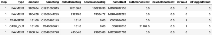
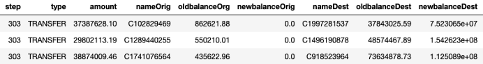
As you can see, we are dealing with both numerical data, such as the ‘amount’ and ‘oldbalanceOrg’ fields, as well as categorical data, such as the ‘type’ and ‘nameOrig’ fields. To the extent that we need to understand the data at hand, the column names should, for the most part, provide enough information about the meaning of the records. In short, each entry deals with information about the original and the new account balance of each of the two parties involved in the transaction (origin and destination), as well as a separate record of the exact amount (supposed to be) transferred. The ‘step’ field denotes the number of hours passed since the start of the simulation.
In addition to the above described transaction records, which are probably not too different from most other datasets of this category, two additional columns are present that relate to the goal of this article: ‘isFraud’ and ‘isFlaggedFraud’. The ‘isFraud’ column tells us which transactions are indeed fraudulent, whereas the ‘isFlaggedFraud’ column is a simple indicator variable for whether the amount transferred in a given transaction exceeds the threshold of 200’000. This latter field represents a very simple fraud detection strategy that belongs to the hard-coded kind mentioned in the introduction of this article.
We will not train our model on either of these two additional fields, since in many real-world cases there will be no prior information available on what kinds of transactions represent fraudulent activity. The ‘isFraud’ column will provide us with ground truth values for whether transactions are fraudulent or not, against which our anomaly detection model can be evaluated. The naive rule that forms the basis for the ‘isFlaggedFraud’ column, namely that transactions with high amounts are more likely to be anomalies, shall be used as a baseline that represents an instance of hard-coded models, which we would like to improve upon.
Feature Engineering
All numerical features can easily be used as inputs to the model, so the fields ‘amount’, ‘oldbalanceOrg’, ‘newbalanceOrig’, ‘oldbalanceDest’ and ‘newbalanceDest’ will be used as features as they are.
features = pd.DataFrame(index=transactions.index)

numerical_columns = ['amount', 'oldbalanceOrg', 'newbalanceOrig', 'oldbalanceDest', 'newbalanceDest']
features[numerical_columns] = transactions[numerical_columns]
Since the ‘amount’ field seems to sometimes deviate from the difference between the original and the new balances of one or both of the transaction parties, we decided to include these differences in the data as two additional features: ‘changebalanceOrig’ and ‘changebalanceDest’.
features[‘changebalanceOrig’] = features[‘newbalanceOrig’] — features[‘oldbalanceOrg’]
features[‘changebalanceDest’] = features[‘newbalanceDest’] — features[‘oldbalanceDest’]
Since the ‘step’ field gives us the relative timestamps of all transactions in an hourly resolution, we can derive the (hourly) time of the day when the transaction occurred. To do this we simply transform the ‘step’ field by applying the modulo of 24.
features[‘hour’] = transactions[‘step’] % 24s
Finally, we want to make use of the information provided in the ‘type’ column. Since our model will only be able to use numerical data, and since there is no logical ordering of the values that the ‘type’ field can assume, we will proceed by one-hot encoding the field into 5 columns, one for each of the possible values of ‘type’. The binary values in the columns indicate whether the content of ‘type’ is equal to the column’s corresponding value. The matrix of one-hot encodings is then appended to our feature matrix.
type_one_hot = pd.get_dummies(transactions[‘type’])
features = pd.concat([features, type_one_hot], axis=1)
Requirements
To function as a fraud detection system that is as general as possible, we want the following properties in our model:
- Makes no assumptions about what an anomaly looks like.
- Does not require any flagged data (labels).
- Provides a continuous anomaly score, such that the number of identified anomalies can be adjusted depending on the desired strictness.
The anomaly detection model we are going to use in this article is the Isolation Forest described in this paper. It fulfills all of the above requirements and relies on two simple assumptions: Anomalies are few, and anomalies are different.
Isolation Forest: Intuition
Isolation Forest assigns an anomaly score to data points based on how easy they are to separate from the rest of the data. The easier a data point is isolated from the majority of the data, the more likely it is to be an anomaly. But how does the model determine whether a point is ‘easier’ to isolate in practice? Simply put, the model tries to isolate points by asking random questions of the following form:
Is feature x larger or smaller than threshold y?
Both feature x and the threshold y are chosen randomly. Given enough random questions, eventually every unique data point will be isolated. Isolation Forest considers points that require more such questions as harder to isolate and thus more likely to be anomalies. To get an intuition for why this works, consider the following two processes of isolation for different data points. Let’s first look at a point that could be considered an anomaly in the sense that there are not many other points similar to it.
It took 12 random questions to completely isolate the point. Now let’s take a look at a data point more towards the center of the distribution that should be less likely to be an anomaly in the sense that there are many points that are similar to it.
For this more ‘normal’ point, 22 decisions were needed to isolate it, many more than for our anomalous point. Clearly, this is subject to a lot of variance, and the actual Isolation Forest model repeats this procedure many times to arrive at a final anomaly score. But this idea of anomalies needing fewer decisions to isolate them lies at the heart of the model.
Implementation
Using scikit-learn’s Isolation Forest implementation, we can create and fit our model in just two lines of code. The default parameters have been shown to perform well in many real-world scenarios, so we will not change anything about the default parameters, except the random state for reproducibility.
from sklearn.ensemble import IsolationForest
forest = IsolationForest(random_state=0)
forest.fit(features)
To get a continous anomaly score for each data point rather than a binary anomaly indicator which would be dependent on an arbitrarily-chosen threshold value, we call the score samples method.
scores = forest.score_samples(features)
Results
The following graph shows the distribution of all the anomaly scores obtained by running the code from the previous section.
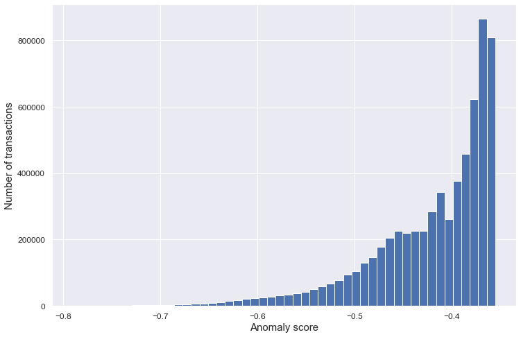
The raw output of the Isolation Forest is not a split of the dataset into anomalies and non-anomalies, but rather a list of continuous anomaly scores, one for every entry. This means that, depending on how many anomalies we want to detect (how wide we want to cast our net), we can set a different threshold which determines the data points that are considered as anomalies (i.e. data points with scores below the threshold). One way to evaluate the result of our model without choosing one particular threshold is by computing the area under the ROC curve of the model output.
To have a baseline to compare the Isolation Forest results to, we chose to evaluate a naive method for anomaly detection which consists of treating the ‘amount’ field as anomaly score, where higher amounts represent a higher chance of being an anomaly. This approach was taken to compute the ‘isFlaggedFraud’ column of the data set as well. We will follow this approach without a fixed threshold to compute a naive ROC curve.
Finally, we will add the ROC curve that would be obtained by random guessing. The predicted anomalies are evaluated against the ‘isFraud’ column, which represents the ground truth value of whether the given entry constitutes an anomaly or not.
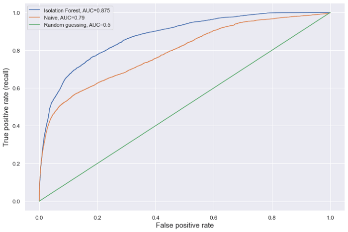
As is visible by the above plot, our Isolation Forest approach clearly exceeds the naive one if we generalize over all possible thresholds. Overall, an AUC of 0.875 is quite promising, especially when considering the fact that we haven’t done any optimization in terms of feature selection or model hyperparameter tuning.
But what can we do now with these results? Since we have a continuous anomaly score for every data point, we could, for instance, decide to look at the top 3 anomalies in our dataset:
This is all well and good, but unless you are very familiar with the data and its distribution, it might not be obvious why these exact data points were selected by the model to be likely candidates for anomalies. Without any interpretation of the output, it is hard for a human expert to decide whether the anomaly found constitutes actual fraudulent activity, or a false positive. This is where the explanation model comes in.
Explanation Model
The explanation model we are going to use for the output of the Isolation Forest is called SHAP, which was introduced in this paper. For our purposes, what we need to understand about SHAP is that the explanation values it provides tell us about the effect that the value of a feature of a particular data point had on its associated anomaly score. In other words, if we look at a particular output of our model, SHAP values tell us how much each feature of the input contributed to that score, and in which direction (i.e. whether the feature contributed to a higher or a lower anomaly score). Before we look at an example to elucidate the nature of SHAP values, let’s take a look at how to compute them using the SHAP library.
First, we need to instantiate an appropriate Explainer model. Since we are using a tree-based model it makes sense to use SHAP’s TreeExplainer
import shap
explainer = shap.TreeExplainer(forest)
Since we could never look at the explanations of every single data point, and since a random subsample can already reveal a lot about our model’s output, we will compute the SHAP values for a set of 5000 randomly chosen data points.
random_indices = np.random.choice(len(features), 5000)
shap_values_random = explainer.shap_values(features.iloc[random_indices, :])
random_features = features.iloc[random_indices, :]
Local Explanations
To visualize the explanation values of a single point, we can use the force_plot function. Let’s display the explanation for the first entry in the randomly chosen dataset.
shap.force_plot(explainer.expected_value, shap_values_random[0, :], random_features.iloc[0, :])
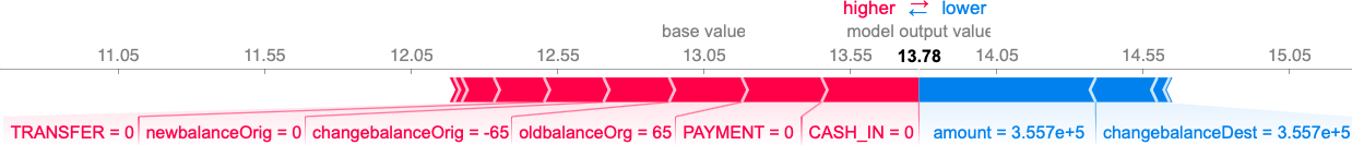
The ‘base value’ in the above plot corresponds to the average output of the model over the training set, whereas ‘model output value’ in bold indicates the model output for this specific datapoint. The purpose of this plot is to show how the individual features of this data point contributed to shifting the model output from its expected (base) value, to the actual value. The values of these individual contributions are SHAP values. Blue bars represent SHAP values that are negative and contributed to a lower anomaly score (making it more likely for that data point to be an anomaly), whereas red bars represent positive SHAP values making the output higher (i.e. suggesting that this data point is normal). The sum of all SHAP values is equal to the difference between base value and model output value. Please note that the SHAP explainer works with raw anomaly scores, whereas on the histogram in the ‘Results’ section we were looking at normalized values. The meaning stays the same: a lower score implies higher chance of being an anomaly.
In the above example we can see that, while a couple of features were suggestive of this data point being anomalous, such as the amount field (presumably because it is a rather high amount), most of the features indicate that this data point is rather normal.
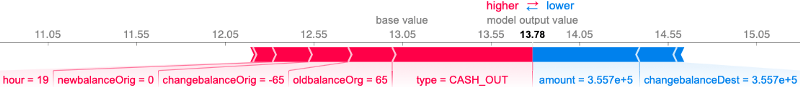
One issue with the previous plot is the fact that the different values of the ‘type’ field are treated as separate features with binary values due to the one-hot-encoding we applied in the beginning. To solve this, we can simply undo the one-hot-encoding in the feature matrix and add all of the corresponding SHAP values to 1 single value. This is possible thanks to the additive nature of SHAP values. The following plot was created by using the adjusted features and SHAP values.
Global Insights
Even though SHAP values are local explanations, i.e. they explain the contributions of features on single data points, we can gain more general insights about the decision our model makes by aggregating many of these local explanations to discover global trends.
One useful tool that the SHAP library provides to gain such insights is the dependence_plot function. It shows us how, across many data points, a SHAP value of a specific feature (y-axis) depends on the feature’s value (x-axis). Dots in the plot represent individual data points.
shap.dependence_plot(
 'changebalanceDest',
 shap_values_random,
 random_features,
 interaction_index=None,
 xmax='percentile(99)'
)
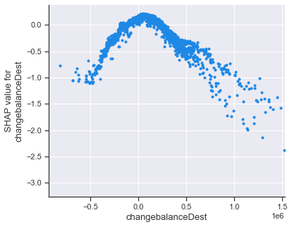
We can see that the SHAP value of ‘changebalanceDest’ is positive for values close to zero, suggesting small changes in the receiver account’s balance are common. The more the absolute value increases, the more the SHAP value contributes to making the anomaly score lower (i.e. increasing the chance of being an anomaly). We can see that the most significant SHAP values are in the realm of very large positive numbers. Thedependence_plot also allows us to take into consideration the effect of another feature with the interaction_index argument.
shap.dependence_plot(
 'changebalanceDest',
 shap_values_random,
 random_features,
 interaction_index='CASH_OUT',
 xmax='percentile(99)'
)
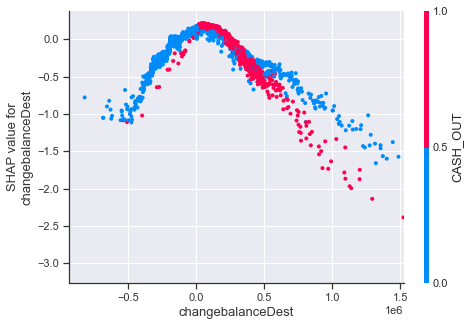
This plot shows that, whether the ‘type’ field of a data point is equal to CASH_OUT or not also correlates with how the SHAP value for ‘changebalanceDest’ behaves. It seems as though large sums of money become indicators for an anomaly more quickly if the ‘type’ field is equal to CASH_OUT.
We can also detect an interesting interaction between the SHAP value of the ‘hour’ feature and whether the ‘type’ feature is equal to PAYMENT.
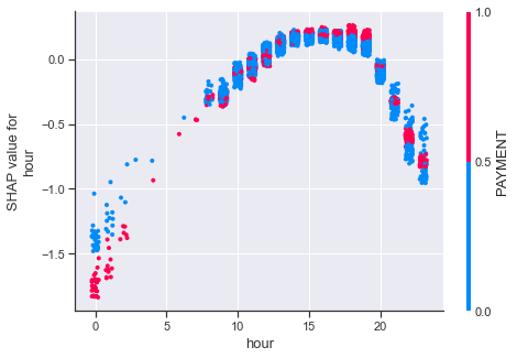
While a ‘hour’ value between 0 and 5 is generally indicative of being an anomaly, this effect is more pronounced for transactions of the PAYMENT type. Interestingly, this effect is not there or even reversed during other times of the day.
Conclusion
Finding fraudulent activity in transaction data can be of significant value to many companies from different industries. In most cases, the sheer size of the data sets require an (at least partially) automated approach. Moreover, the complexity of the data makes it difficult to devise hard-coded rules that anticipate all possible types of anomalies that could occur. Given these challenges, unsupervised machine learning is a fitting first approach to tackle the problem of fraud detection, and Isolation Forest represents a powerful member of this family of ML algorithms that can be used for outlier detection. By using the Paysim dataset as an example, we showed how transaction data can be pre-processed and how sklearn’s implementation of the Isolation Forest can be used to achieve accurate outlier scores on this data. Moreover, we briefly introduced SHAP values to explain these outlier scores, both at the level of local explanations and at the global level of general trends that are present in our anomaly detection model. These explanations can inform experts about the validity of the produced outlier scores, as well as provide insights into what other features could be included to improve performance. The generality of this approach should make it easy to adapt this procedure for many different transaction data sets.
Interested to learn more? See a webinar on fraud detection by Francesco Lässig and Maxime Dumonal.
