
- Jul 6, 2021
- 16 min read
Written By
- Francesco Lässig
How a convolutional network with some simple adaptations can become a powerful tool for sequence modeling and forecasting.
Although commonly associated with image classification tasks, convolutional neural networks (CNNs) have proven to be valuable tools for sequence modeling and forecasting, given the right modifications. In this article we explore in detail the basic building blocks that a Temporal Convolutional Network (TCN) consists of, and how they all fit together to create a powerful forecasting model. Using our open-source Darts TCN implementation, we show that accurate predictions can be achieved on a real-world dataset with only a few lines of code.
The following description of a Temporal Convolutional Network is based on the following paper: https://arxiv.org/pdf/1803.01271.pdf. References to this paper will be denoted by (*).
Motivation
Up until recently, the topic of sequence modeling in the context of deep learning has been largely associated with recurrent neural network architectures such as LSTM and GRU. S. Bai et al. (*) suggest that this way of thinking is antiquated, and that convolutional networks should be taken into consideration as one of the primary candidates when modeling sequential data. They were able to show that convolutional networks can achieve better performance than RNNs in many tasks while avoiding common drawbacks of recurrent models, such as the exploding/vanishing gradient problem or lacking memory retention. Furthermore, using a convolutional network instead of a recurrent one can lead to performance improvements as it allows for parallel computation of outputs. The architecture they propose is called Temporal Convolutional Network (TCN) and will be explained in the following sections. To facilitate understanding the TCN architecture in conjunction with its Darts implementation, this article will use the same model parameter names as seen in the library wherever possible (indicated in bold).
Overview
A TCN, short for Temporal Convolutional Network, consists of dilated, causal 1D convolutional layers with the same input and output lengths. The following sections go into detail about what these terms actually mean.
1D Convolutional Network
A 1D convolutional network takes as input a 3-dimensional tensor and also outputs a 3-dimensional tensor. The input tensor of our TCN implementation has the shape (batch_size, input_length, input_size) and the output tensor has the shape (batch_size, input_length, output_size). Since every layer in a TCN has the same input and output length, only the third dimension of the input and output tensors differs. In the univariate case, input_size and output_size will both be equal to one. In the more general multivariate case, input_size and output_size might differ since we might not want to forecast every component of the input sequence.
One single 1D convolutional layer receives an input tensor of shape (batch_size, input_length, nr_input_channels) and outputs a tensor of shape (batch_size, input_length, nr_output_channels). To see how one single layer converts its input into the output, let’s look at one element of the batch (the same process takes place for every element in the batch). Let’s start with the simplest case where nr_input_channels and nr_output_channels both equal 1. In this case we are looking at 1D input and output tensors. The following image shows how one element of the output tensor is computed.
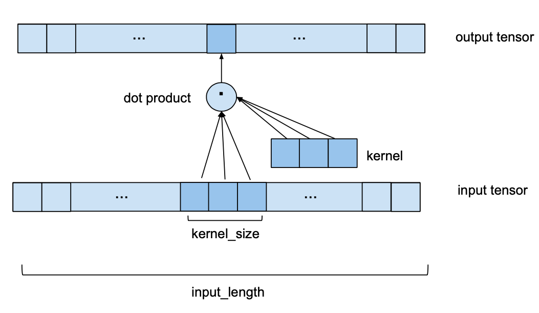
We can see that to compute one element of the output, we look at a series of consecutive elements of length kernel_size of the input. In the above example we chose a kernel_size of 3. To obtain the output, we take the dot product of the subsequence of the input and a kernel vector of learned weights of the same length. To get the next element of the output, the same procedure is applied, but the kernel_size-sized window of the input sequence is shifted to the right by one element (for the purposes of this forecasting model, the stride is always set to 1). Please note that the same set of kernel weights will be used to compute every output of one convolutional layer. The following image shows two consecutive output elements and their respective input subsequences.
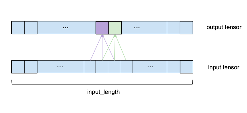
To make the visualization simpler, the dot product with the kernel vector is not shown anymore, but takes place for every output element with the same kernel weights.
To make sure that the output sequence has the same length as the input sequence, some zero-padding is applied. This means that additional zero-valued entries are added to either the beginning or the end of the input tensor to ensure that the output has the desired length. How this is done exactly will be explained in later sections.
Now let’s look at the case where we have multiple input channels, i.e. nr_input_channels is larger than 1. In this case, the process described above is repeated for every single input channel, but each time with a different kernel. This leads to nr_input_channels intermediate output vectors and a number of kernel weights of kernel_size * nr_input_channels. Then, all the intermediate output vectors are summed up to obtain the final output vector. In some sense this is equivalent to a 2D convolution with an input tensor of shape (input_size, nr_input_channels) and a kernel of shape (kernel_size, nr_input_channels) as shown in the following image. It’s still 1D in the sense that the window only moves along a single axis, but we do have a 2D convolution at every step in the sense that we are using a 2-dimensional kernel matrix.
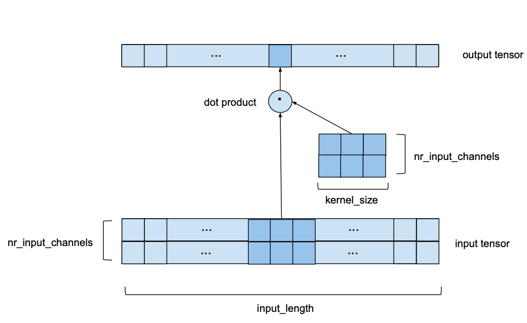
For this example we chose nr_input_channels to be equal to 2. Now, instead of a kernel vector sliding over a 1-dimensional input sequence we have a nr_input_channels by kernel_size kernel matrix sliding along a nr_input_channels wide series of length input_length.
If both nr_input_channels and nr_output_channels are larger than 1, the above process is simply repeated for every output channel with a different kernel matrix. The output vectors are then stacked on top of each other resulting in an output tensor of shape (input_length, nr_output_channels). The number of kernel weights in this case is equal to kernel_size*nr_input_channels*nr_output_channels.
The two variables nr_input_channels and nr_output_channels depend on the position of the layer within the network. The first layer will have nr_input_channels = input_size, and the last layer will have nr_output_channels = output_size. All other layers will use the intermediate channel number given by num_filters.
Causal Convolution
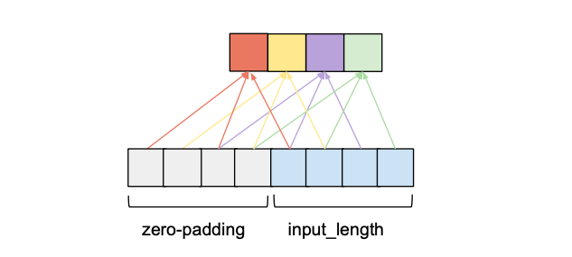
For a convolutional layer to be causal, for every i in {0, …, input_length — 1} the i’th element of the output sequence may only depend on the elements of the input sequence with indices {0, …, i}. In other words, an element in the output sequence can only depend on elements that come before it in the input sequence. As mentioned before, to ensure an output tensor has the same length as the input tensor, we need to apply zero padding. If we only apply zero-padding on the left side of the input tensor, then causal convolution will be ensured. To understand this, consider the rightmost output element. Given that there is no padding on the right side of the input sequence, the last element it depends on is the last element of the input. Now consider the second to last output element of the output sequence. Its kernel window is shifted to the left by one compared to the last output element, that means its rightmost dependency in the input sequence is the second to last element of the input sequence. It follows by induction that for every element in the output sequence, its latest dependency in the input sequence has the same index as itself. The following figure shows an example with an input_length of 4 and a kernel_size of 3.
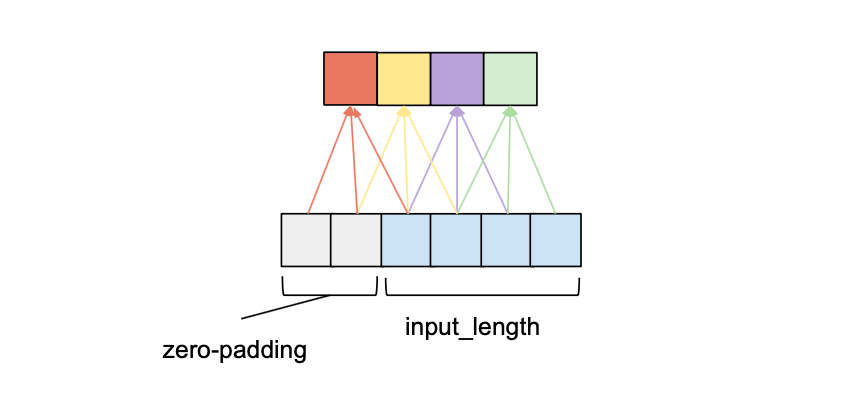
We can see that with a left zero-padding of 2 entries we can achieve the same output length while obeying the causality rule. In fact, without dilation, the number of zero-padding entries required for maintaining the input length is always equal to kernel_size – 1.
Dilation
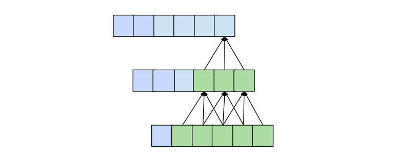
One desirable quality of a forecasting model is that the value of a specific entry in the output depends on all previous entries in the input, i.e. all entries that have an index smaller or equal to itself. This is achieved when the receptive field, meaning the set of entries of the original input that affect a specific entry of the output, has size input_length. We also call this ‘full history coverage’. As we have seen before, one conventional convolutional layer makes an entry in the output dependent on the kernel_size entries of the input that have an index smaller or equal to itself. For instance, if we have a kernel_size of 3, the 5th element in the output will be dependent on elements 3, 4 and 5 of the input. This reach is expanded when we stack multiple layers on top of each other. In the following figure we can see that by stacking two layers with kernel_size 3 we get a receptive field size of 5.
More generally, a 1D convolutional network with n layers and a kernel_sizek has a receptive field r of size

To know how many layers are needed for full coverage, we can set the receptive field size to input_length l and solve for the number of layers n (we need to round up in case of non-integer values):

This means that, given a fixed kernel_size, the number of layers required for full history coverage is linear in the length of the input tensor, which will result in networks that become very deep very fast, leading to models with a very large number of parameters that take longer to train. Furthermore, a high number of layers has been shown to lead to degradation problems related to the gradient of the loss function. One way to increase the receptive field size while still keeping the number of layers relatively small is to introduce dilation to the convolutional network.
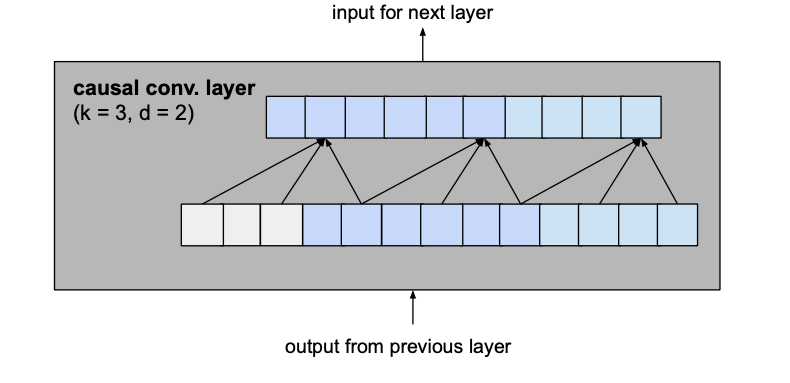
Dilation in the context of a convolutional layer refers to the distance between the elements of the input sequence that are used to compute one entry of the output sequence. So a conventional convolutional layer could be seen as a 1-dilated layer, since the input elements for 1 output value are adjacent. The following figure shows an example of a 2-dilated layer with an input_length of 4 and a kernel_size of 3.
Compared to the 1-dilated case, this layer has a receptive field that spreads across a length of 5 rather than 3. More generally, a d-dilated layer with a kernel size k has a receptive field spreading across a length of 1+d*(k-1). If d is fixed, this will still require a number linear in the length of the input tensor to achieve full receptive field coverage (we just decreased the constant).
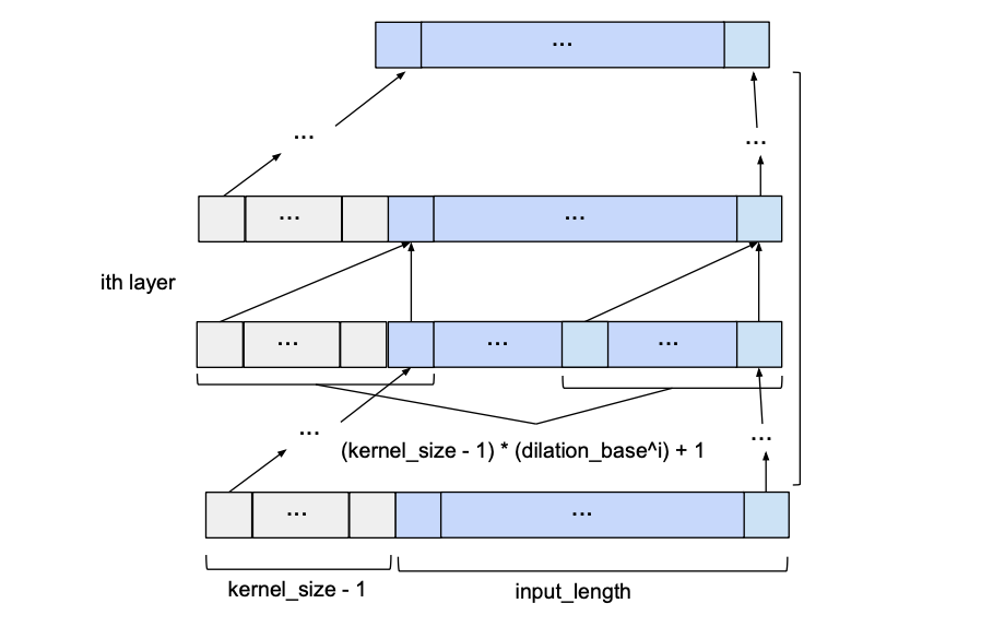
This problem can be addressed by increasing the value of d exponentially as we move up through the layers. For this, we choose a constant dilation_base integer b which will let us compute the dilation d of a specific layer as a function of the number of layers below it, i, as d = b**i. The following figure shows a network with an input_length of 10, a kernel_size of 3 and a dilation_base of 2 which results in 3 dilated convolutional layers for full coverage.
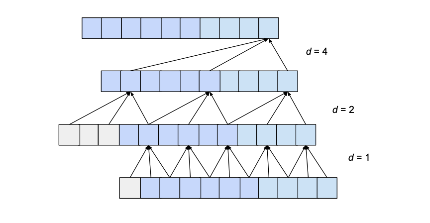
Here we only show the influence of inputs that affect the last value of the output. Likewise, only zero-padding entries necessary for the last output value are shown. Clearly, the last output value is dependent on the whole input coverage. Actually, given the hyperparameters, an input_length of up to 15 could be used while maintaining full receptive field coverage. Generally speaking, every additional layer adds a value of d*(k-1) to the current receptive field width, where d is computed as d=b**i, with irepresenting the number of layers below our new layer. Consequently, the width of the receptive field w of a TCN with exponential dilation of base b, kernel size k and number of layers n is given by

However, depending on the values b and k, this receptive field can have ‘holes’. Consider the following network with a dilation_base of 3 and a kernel size of 2:
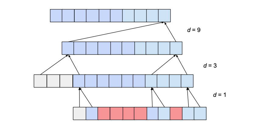
The receptive field does cover a range that is larger than the input size (namely 15). However, the receptive field has holes in it; that is there are entries in the input sequence that the output value is not dependent on (shown above in red). To solve this problem, we need to either increase the kernel size to 3, or decrease the dilation base to 2. Generally speaking, for a receptive field with no holes, the kernel size k has to be at least as big as the dilation base b.
Considering these observations, we can compute how many layers our network needs for full history coverage. Given a kernel size k, dilation base b, where k ≥ b, and input length l, the following inequality must hold for full history coverage:

We can solve for n and get the minimum number of required layers as

We can see that the number of layers is now logarithmic rather than linear in the length of the input. This constitutes a significant improvement, which can be achieved without sacrificing receptive field coverage.
Now the only thing left to specify is the number of zero-padding entries required at each layer. Given a dilation base b, a kernel size k and a number of i layers below our current layer, then the number of zero-padding entries p needed for the current layer are computed as follows:

Basic TCN Overview
Given input_length, kernel_size, dilation_base and the minimum number of layers required for full history coverage, the basic TCN network would look something like this:
Forecasting
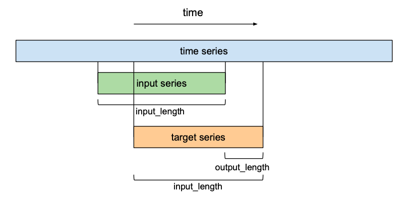
So far we have only talked about the ‘input sequence’ and the ‘output sequence’ without getting into how they relate to each other. In the context of forecasting, we want to predict the next entries of a time series into the future. To train our TCN network to do forecasting, the training set will consist of (input sequence, target sequence)-pairs of equally-sized subsequences of the given time series. A target series will be a series that is shifted forward in relation to its respective input series by a certain number output_length. This means that a target series of length input_lengthcontains the last (input_length – output_length) elements of its respective input sequence as first elements, and the output_length elements that come after the last entry of the input series as its final elements. In the context of forecasting, this means that the maximum forecasting horizon that can be predicted with such a model is equal to output_length. Using a sliding window approach, many overlapping pairs of input and target sequences can be created out of one time series.
Improvements to the Model
S. Bai et al. (*) suggest a few additions to the basic TCN architecture for improved performance which will be discussed in this section, namely residual connections, regularization and activation functions.
Residual Blocks
The biggest modification we make to the previously introduced basic model is to change the fundamental building block of the model from a simple 1D causal convolutional layer to a residual block which consists of 2 layers with the same dilation factor and a residual connection.
Let’s consider a layer with a dilation factor d of 2 and kernel size k of 3 from the basic model to see how this translates into a residual block of the improved model.
becomes
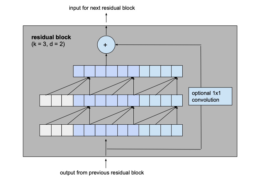
The output of the two convolutional layers will be added to the input of the residual block to produce the input for the next block. For all inner blocks of the network, i.e. all but the first and the last one, the input and output channel width is the same, namely num_filters. Since the first convolutional layer of the first residual block and the second convolutional layer of the last residual block may have different input and output channel widths, the width of the residual tensor might have to be adjusted, which is done using a 1×1 convolution.
This change affects the calculus for the minimum number of required layers for full coverage. Now we have to think about how many residual blocks are necessary to achieve a full receptive field coverage. Adding a residual block to a TCN adds twice as much receptive field width than when adding a basic causal layer, since it includes 2 such layers. So the total size of the receptive field r of a TCN with dilation base b, kernel size k with k ≥ b and number of residual blocks n can be computed as

which leads to a minimum number of residual blocks n for full history coverage of input_length l of

Activation, Normalization, Regularization
To make our TCN more than just an overly complex linear regression model, activation functions need to be added on top of the convolutional layers to introduce non-linearities. ReLU activations are added to the residual blocks after both convolutional layers.
To normalize the input of hidden layers (which counteracts the exploding gradient problem among other things), weight normalization is applied to every convolutional layer.
In order to prevent overfitting, regularization is introduced via dropout after every convolutional layer in every residual block. The following figure shows the final residual block.
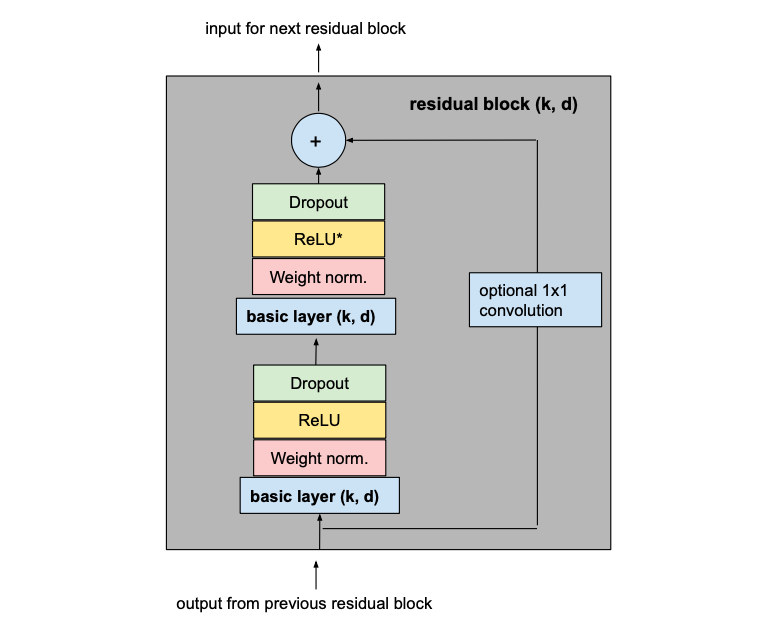
The asterisk in the second ReLU unit indicates that it is present in every layer but the last one, since we want our final output to be able to take on negative values as well (this differs from the architecture outlined in the paper).
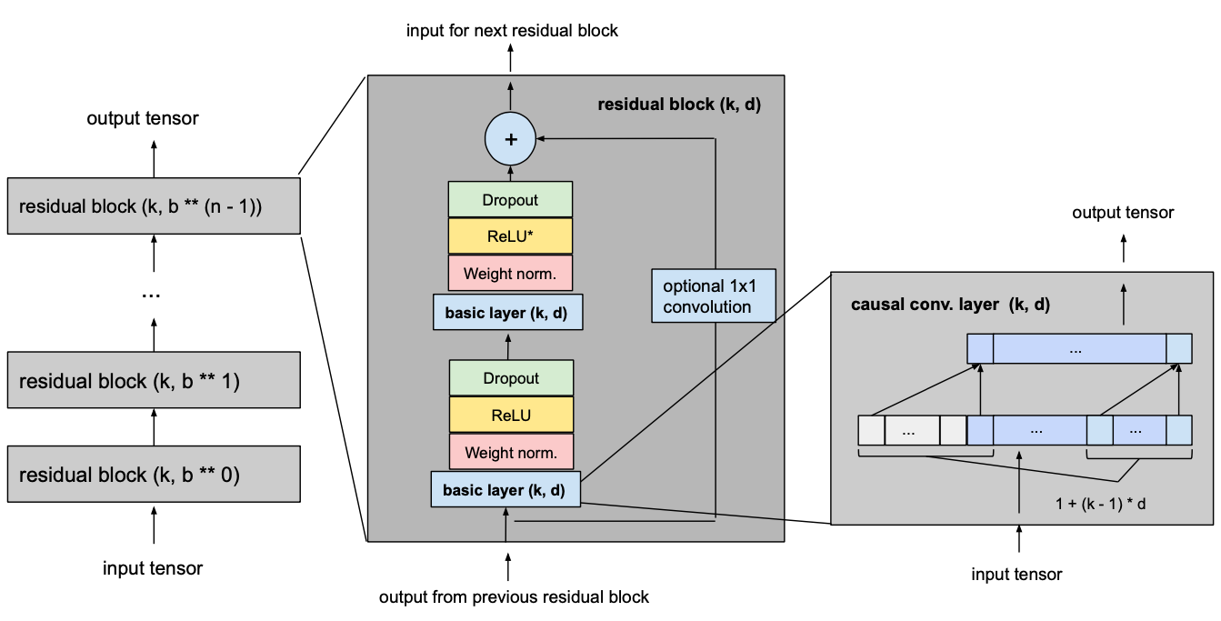
Final Model
The following picture shows our final TCN model with l equal to input_length, k equal to kernel_size, b equal to dilation_base, k ≥ b and with a minimum number of residual blocks for full history coverage n,where n can be computed from the other values as explained above.
Example
Let’s take a look at an example of how we can use the TCN architecture to forecast a time series using the Darts library.
First, we need a time series to train and evaluate our model on. For this, we use a Kaggle dataset containing hourly energy production data from Spain. More specifically, we choose to predict the ‘run-of-river hydroelectricity’ production. Furthermore, to make the problem less computation-intensive, we average the energy production over each day to get a daily time series.
from darts import TimeSeries
from darts.dataprocessing.transformers import
MissingValuesFiller
import pandas as pd

df = pd.read_csv('energy_dataset.csv', delimiter=",")
df['time'] = pd.to_datetime(df['time'], utc=True)
df['time']= df.time.dt.tz_localize(None)

df_day_avg =
df.groupby(df['time'].astype(str).str.split(" ").str[0]).mean().reset_index()

value_filler = MissingValuesFiller()
series =
value_filler.transform(TimeSeries.from_dataframe(df_day_avg, 'time', ['generation hydro run-of-river and poundage']))

series.plot()
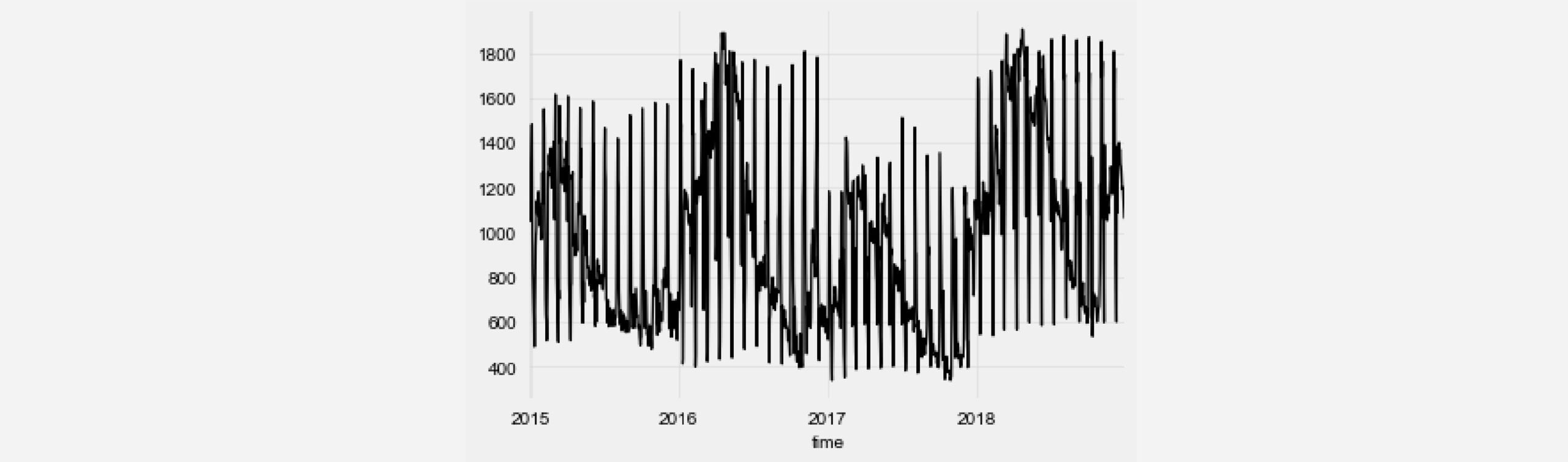
We can see that, in addition to a yearly seasonality, there are regular ‘spikes’ in energy production that come in monthly intervals. Since the TCN model supports multiple input channels, we can add additional time series components to the current time series that encode the current day of the month. This can help our TCN model to converge faster.
series = series.add_datetime_attribute('day', one_hot=True)
Now we split our data into train and validation components and perform standardization.
from darts.dataprocessing.transformers import Scaler

train, val =
series.split_after(pd.Timestamp('20170901'))

scaler = Scaler()
train_transformed = scaler.fit_transform(train)
val_transformed = scaler.transform(val)
series_transformed = scaler.transform(series)
Now it’s time to create and train our TCN model. Note that all bold variable names that have appeared in the above description of the architecture can be used as arguments for the constructor of the Darts TCN implementation. The output_length parameter is set to 7 since we want to perform weekly forecasts. When training the model, we specify as target_series only the first component of our training series, since we do not want to predict the helper time series we added earlier. We tried out a few different hyperparameter combinations, but most of the values were chosen quite arbitrarily.
from darts.models import TCNModel

model = TCNModel(
    input_size=train.width,
    n_epochs=20,
    input_length=365,
    output_length=7,
    dropout=0,
    dilation_base=2,
    weight_norm=True,
    kernel_size=7,
    num_filters=4,
    random_state=0
)

model.fit(
    training_series=train_transformed,
    target_series=train_transformed['0'],
    val_training_series=val_transformed,
    val_target_series=val_transformed['0'],
verbose=True
)
To evaluate our model, we want to test its performance using a 7-day forecasting horizon on many different points in time in the validation set. For this, we use the historic backtesting functionality from Darts. Note that the model is provided new input data for every prediciton, but it is never retrained. To save time, we set the stride to 5.
pred_series = model.backtest(
    series_transformed,
    target_series=series_transformed['0'],
    start=pd.Timestamp('20170901'),
    forecast_horizon=7,
    stride=5,
    retrain=False,
    verbose=True,
    use_full_output_length=True
)
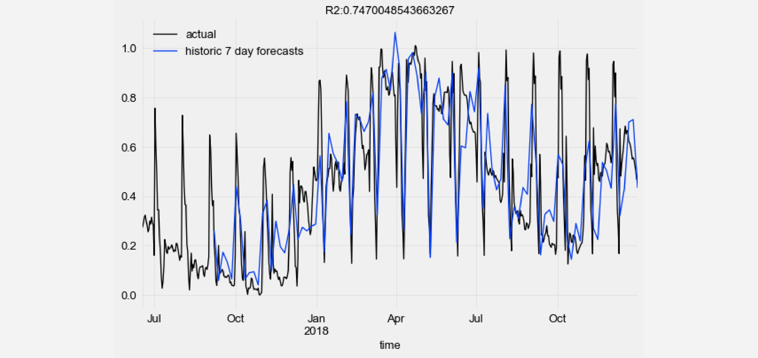
Let’s visualize the historic forecast predictions of our TCN model against the ground truth data points and compute the R2 score.
from darts.metrics import r2_score
import matplotlib.pyplot as plt

series_transformed[900:]['0'].plot(label='actual')
pred_series.plot(label=('historic 7 day forecasts'))
r2_score_value = r2_score(series_transformed['0'], pred_series)

plt.title('R2:' + str(r2_score_value))
plt.legend()
For more details and additional examples, please check out our TCN examples notebook on GitHub.
Conclusion
Deep learning in sequence modeling is, for the most part, still widely associated with recurrent neural network architectures. But research has shown that these types of models can be outperformed in many tasks by a TCN, both in terms of predictive performance and efficiency. In this article we explored how this promising model can be understood in terms of simple building blocks such as 1D convolutional layers, dilations and residual connections, and how they all fit together. Furthermore, we successfully applied the current Darts implementation of the TCN architecture to predict a real-world time series.
Thanks to Julien Herzen.
